
Background
Wilder Blean is a wilding project at West Blean and Thornden Woods, near Canterbury, Kent, UK. The surrounding Blean woodland complex is one of the largest surviving blocks of ancient semi-natural woodland in England (Forestry Commission, 1998). Wilder Blean currently covers an area of 561.8 hectares, comprising a mosaic of ancient oak-hornbeam woodland, mixed broad-leaved coppice with standards, extensive stands of sweet chestnut coppice, conifer plantations, and small areas of heath and wetland as well as several man-made ponds.
Large grazing herbivores, including European bison Bison bonasus, Exmoor ponies Equus ferus caballus, British longhorn cattle Bos primigenius, and Iron Age pigs Sus scrofa × Sus domesticus, were introduced at Wilder Blean in 2022. This is a trial with the aim of improving the condition of the nationally important Site of Special Scientific Interest, some of which is in unfavourable condition (Natural England, 2025).
Large grazing herbivores went extinct in the UK, and across much of Europe, during the late Holocene at the end of the last Ice Age due to a combination of human activity and environmental changes. This was detrimental to the ecosystems in which they evolved, as the functions they provided were lost and natural processes they facilitated were disrupted. Large herbivores control plant growth, maintaining habitat mosaics which support more species, and they disperse seeds that they consume. They create microhabitats by disturbing the ground through trampling, dust bathing or wallowing. They recycle nutrients from plants back into the soils through their dung. They are prey for large predators and scavengers, and support birds and invertebrates that use them as hosts, their dung for food, or their fur for nesting materials. They sequester carbon into soils by depositing their dung and encouraging new rapid plant growth (Borer and Risch, 2024).
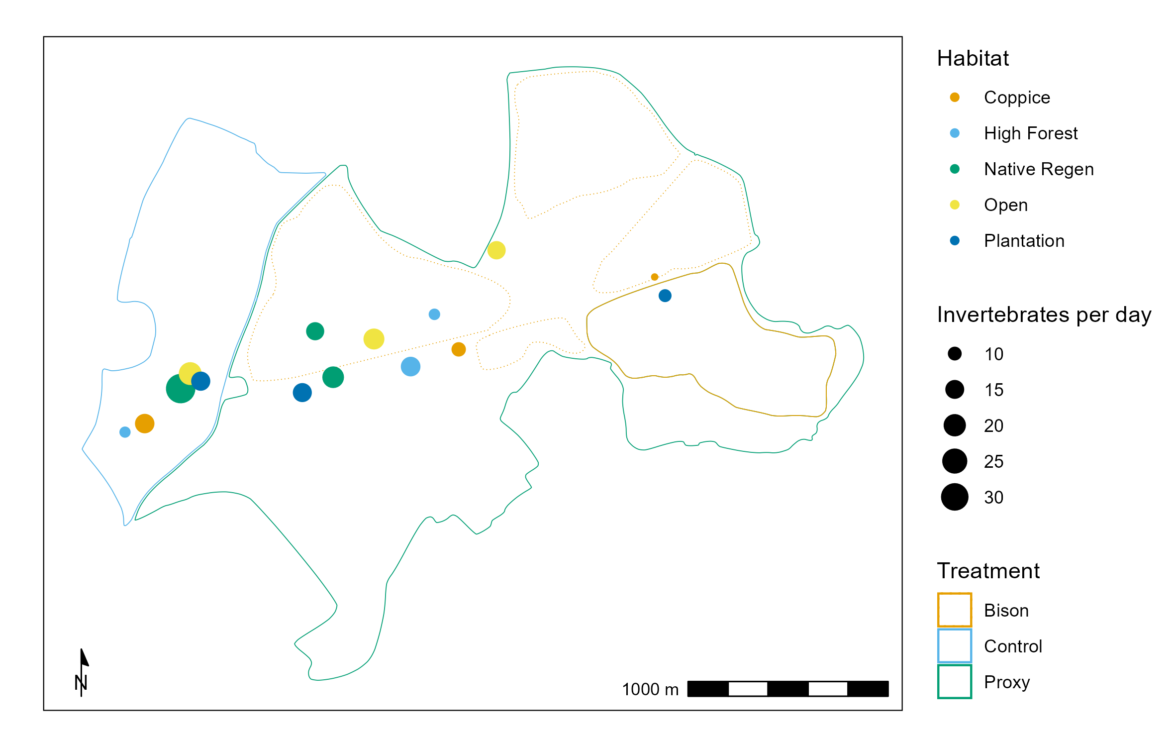
At Wilder Blean, the large herbivores have been reintroduced, but their dispersal is limited by fences. Fencing was required by law under the Dangerous Wild Animals Act 1976, which mandates secure containment for species classified as dangerous to the public. The fences separate the bison from public footpaths and bridleways. The fences are arranged to provide a robust experimental design, comprising three different treatments. The bison treatment area contains European bison. The proxy, or conservation grazers treatment area, contains British longhorn battle, Exmoor ponies and Iron Age pigs. The control treatment area contains no introduced grazing animals and is managed by a human workforce, including coppicing, for example.
This design enables a comparison of the effects of European bison, livestock commonly used for conservation purposes, and traditional human management on the ecosystem, to generate evidence on the effectiveness of European bison as a conservation management tool.
This report summarises the results of the invertebrate surveys conducted between 2021 and 2024.
Methodology
Fifteen Sea, Land and Air Malaise (SLAM) traps were deployed and serviced for five months (May-September) in each year of 2021-2024 at a height of two meters, suspended in trees out of reach of livestock. Five traps were placed in each treatment area, with placement further stratified by habitat type (Coppice, Plantation, High Forest, Open, and Native Regeneration). Unfortunately, due to the delayed construction of the bison tunnels, only one trap was within the bison treatment (Figure 1). Collection periods ranged from 21 to 58 days, with a mean of 31 days. Several traps failed due to vandalism, theft or bad weather.
The invertebrates were preserved in propylene glycol and each trap was serviced once a month with new sample bottles and a fresh batch of propylene glycol left in situ. In the Autumn-Winter following each survey season, volunteers identified all invertebrates to taxonomic Order, and recorded the numbers of each group on a database.
We used a linear mixed-effects model (Bates et al., 2015) in R Studio to assess the effects of treatment type on the collection rate (number of invertebrates trapped per day), while accounting for random variation associated with service date and habitat type. Including service date and habitat type as random effects, means the model includes a random intercept for traps within the same habitat type and a random intercept for each service date, and thus this grouped data structure is acknowledged in the model, improving its accuracy. Satterthwaite’s approximation was used for p-values. The same type of statistical model was also used to test how the collection rate varied by habitat type and service date.
Likelihood ratio tests were used to determine whether adding the fixed effect significantly improved model fit. Post-hoc estimated marginal means (EMMs) were used for pairwise comparisons of collection rates by treatment and habitat type. The response variable, collection rate (in units of invertebrates per day), was log-transformed prior to the analysis to reduce skewness and conform to normality. The results were back-transformed to aid interpretation.
Results
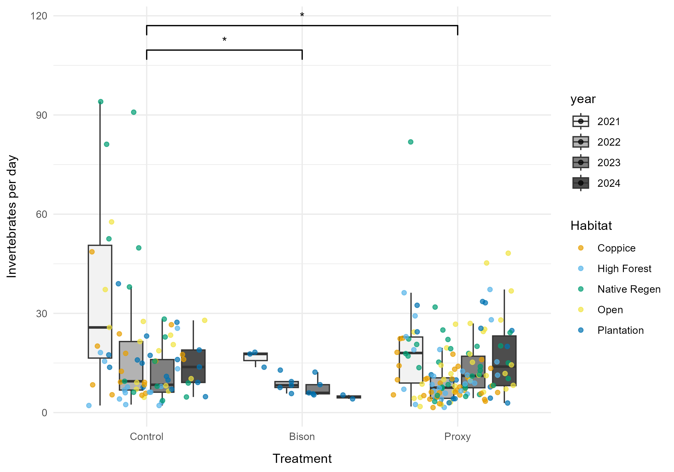
The first model revealed a significant effect of treatment on the invertebrate collection rate (χ2 = 7.8, p = 0.021). The model's marginal R² value was 0.024, indicating that treatment explains 2.4% of the variation in collection rate. The random effects (habitat and service date) explained 32.2% of the variance. The control treatment had the highest collection rate (13.06 ± 2.02 SE invertebrates/day), followed by proxy (10.46 ± 1.53 SE invertebrates/day), and then bison (8.59 ± 2.05 SE invertebrates/day). The collection rate in the bison treatment was 34% lower than the control (p = 0.049). The collection rate in the conservation grazers treatment was 20% lower than the control (p = 0.019) (Figure 2).
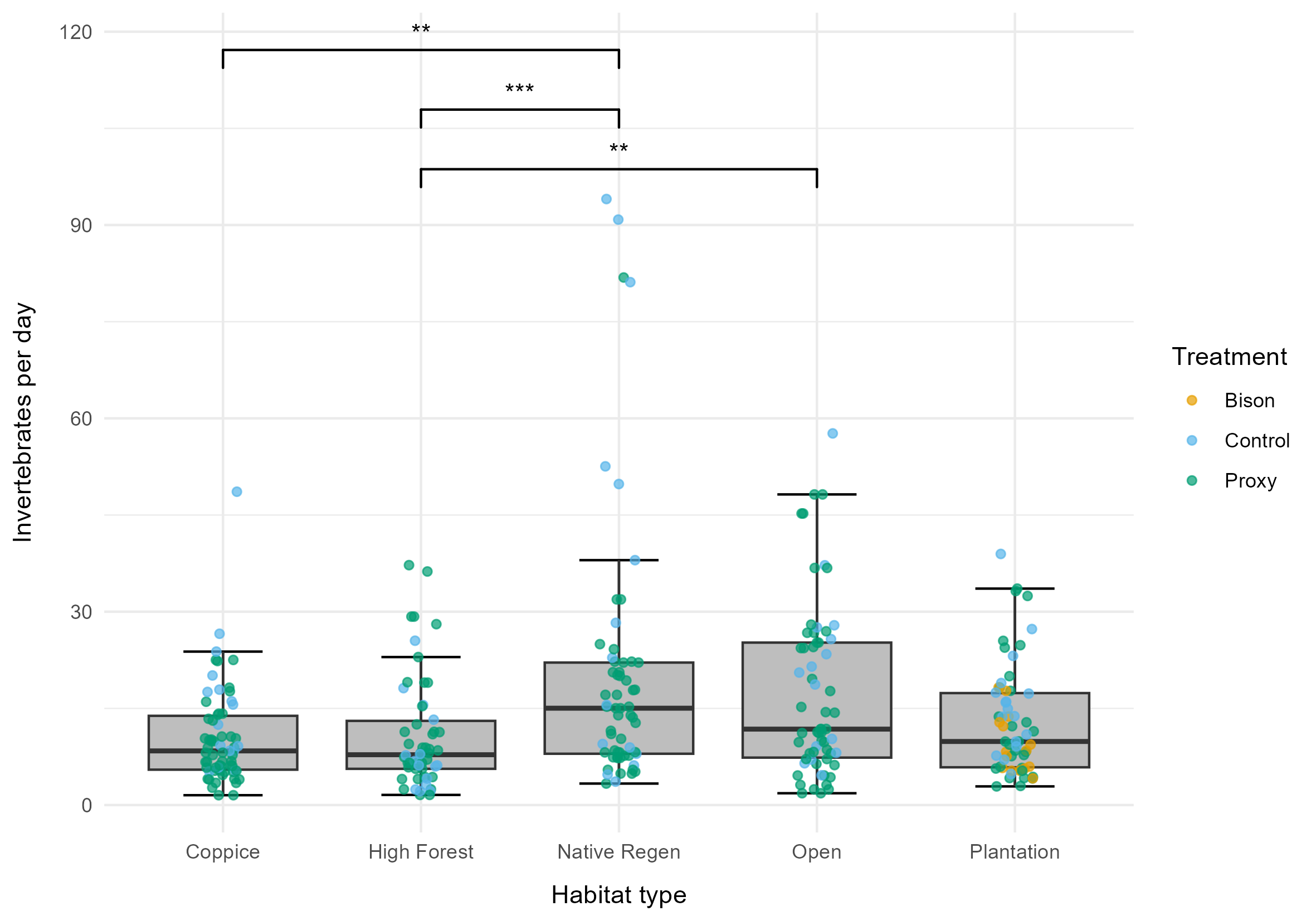
Another model showed that habitat significantly influenced the collection rate (χ2 = 25.6, p <0.001). The model's marginal R² value was 0.079, indicating that habitat explains 7.9% of the variation in collection rate. The random effects (treatment and service date) explained 33.0% of the variance. Collection rates were highest in the native regeneration habitat (15.02 ± 2.57 SE invertebrates/day), followed by open habitat (12.86 ± 2.19 SE invertebrates/day), and lowest in high forest (8.07 ± 1.39 SE invertebrates/day). Pairwise comparisons of estimated marginal means determined that the invertebrate collection rate was 60% higher in native regeneration than coppice (p = 0.002), and 54% higher in native regeneration than high forest (p < 0.001). Additionally, collection rates were 63% higher in open habitat than high forest (p = 0.009). No other pairwise comparisons were statistically significant after adjustment for multiple comparisons (Figure 3).
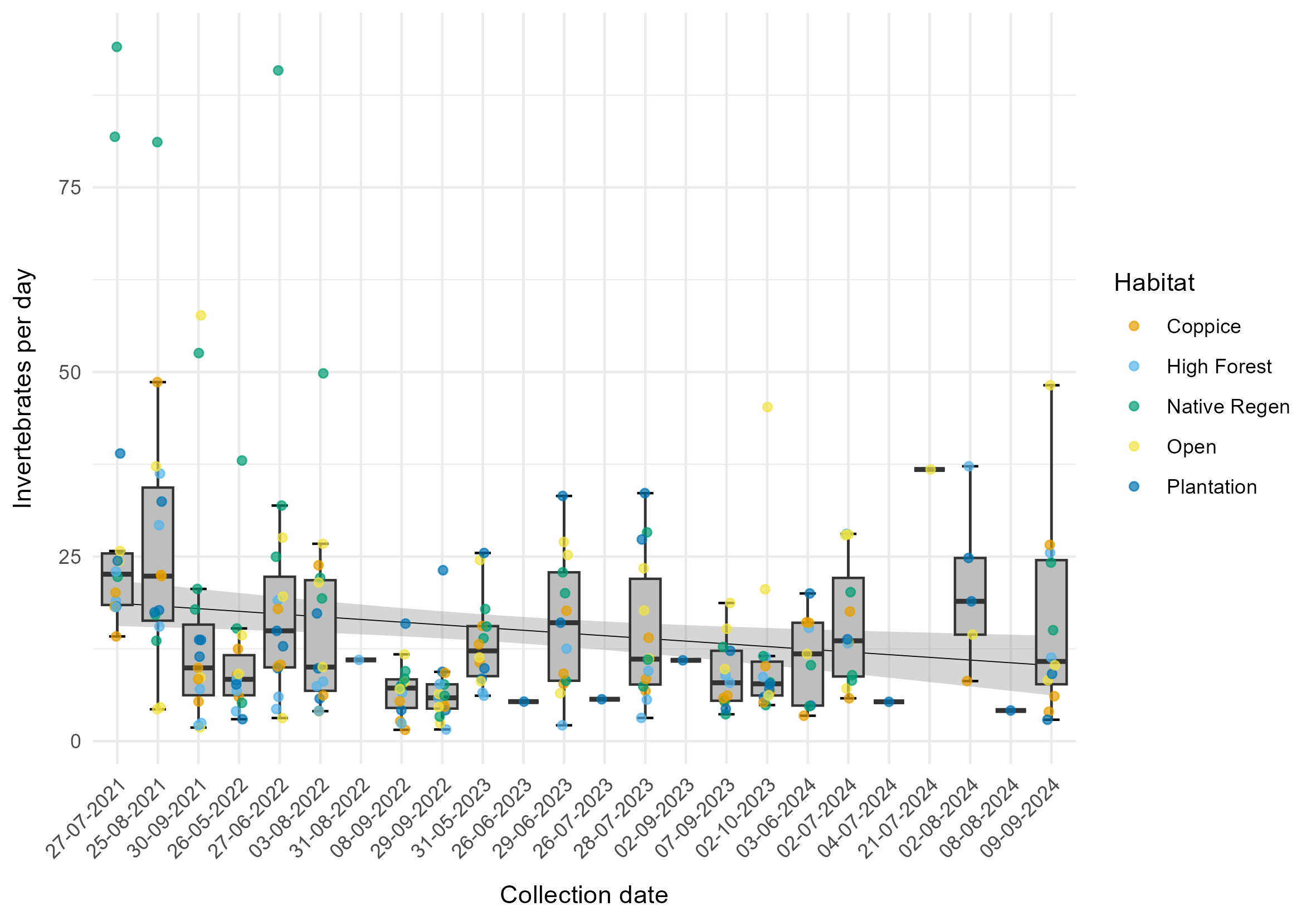
The third model identified a mean decrease in collection rate of approximately 8.7% per year (0.025% ± 0.014% SE per day) but this result was not statistically significant (χ2 = 3.31, p = 0.069). The intercept shows an estimated mean collection rate of 12.51 invertebrates per day (± 1.19 SE) on the first day of sampling. The model's marginal R² value was 0.013, indicating that collection date explains 1.3% of the variation in collection rate. The random effects (treatment and habitat) explained 13.3% of the variance.
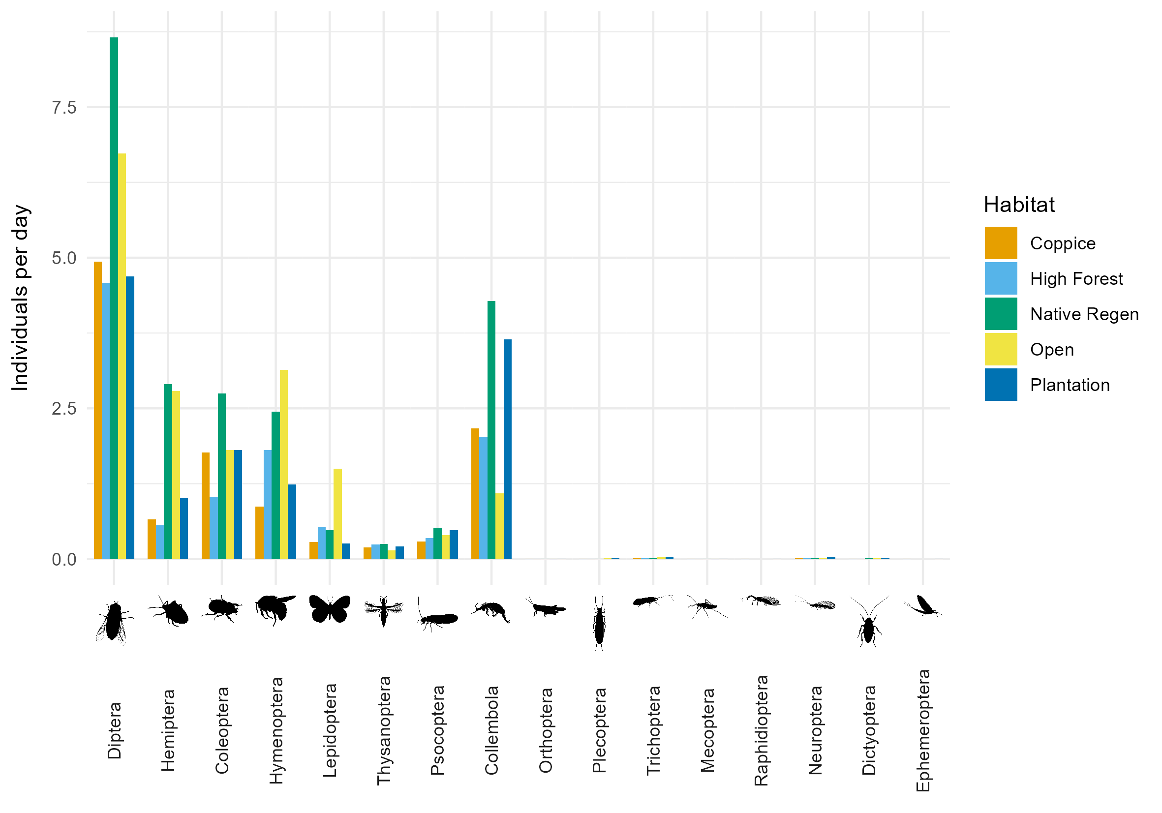
Overall, collection rates were highest for Diptera, Collembola, Hemiptera, Coleoptera and Hymenoptera (Figure 5). Collection rates of Diptera, Hemiptera, Coleoptera and Collembola were highest in native regeneration. Collection rates of Hymenoptera and Lepidoptera were highest in open areas. High forest and plantation had relatively low collection rates across all insect orders, apart from Collembola which were abundant in plantation.
Discussion
The control treatment had higher collection rates than the bison and conservation grazer treatments. This is likely due to the greater areas of open, coppiced and regenerating woodland and areas of heather and bramble-dominated scrub. The bison area has much pine plantation and mature broadleaved woodland. Over time, the conservation grazers and bison should create more open habitat increasing invertebrate abundance in the high forest and plantation.
Native regeneration had the highest collection rates, and significantly higher rates than coppice and high forest. Native regeneration areas have mixed-age trees which provide a complex woodland structure and greater range of invertebrate microhabitats. Moreover, higher light levels reaching the forest floor will increase the temperature, understorey productivity and nectar sources, attracting higher invertebrate numbers, especially pollinators. Unlike coppice, native regeneration will have higher quantities of deadwood supporting detritivorous invertebrates, and also less disturbance.
Additionally, collection rates were higher in open habitat than high forest. Greater direct sunlight and warmth in open areas encourages a greater abundance of herbaceous plants and flowers, and a higher overall plant diversity including grasses, forbs, and early successional species. Greater invertebrate abundance in open habitats compared to closed woodlands is well-documented in temperate Europe (Ball et al., 2024, Dennis, 1997).
The annual decrease in collection rate was 8.7%. Similar declines in insect abundance have been recorded in Kent, and across the UK, over the same time period by the Bugs Matter citizen science survey of insect splats on vehicle number plates (Ball et al., 2023). A growing body of evidence (Hallmann et al., 2017; Goulson, D. 2019; Sánchez-Bayo and Wyckhuys, 2019; Thomas et al., 2019; van der Sluijs, 2020; Outhwaite et al., 2022) highlights population declines in insects and other invertebrates at UK and global scales. The observed decrease could be the result of both a long-term background rate of decline and short-term reduced insect abundance because of the extreme hot and dry climate in the UK in the summer of 2022 and spring of 2023.
The delayed construction of the bison tunnels meant that the bison treatment was not applied according to the experimental design. Between 2021-2024, the bison have been restricted to the South East bison compartment, where only a single trap was deployed, and in 2024 it failed. Therefore the bison treatment results must be interpreted with caution and treated as a baseline at this stage. With the construction of two tunnels now complete, we will see the bison occupying two new compartments in 2025, and the additional compartments in 2026.
References
Ball L, Whitehouse A, Bowen-Jones E, Amor M, Banfield N, Hadaway P & Hetherington P (2023). The 2023 Report: The Bugs Matter Citizen Science Survey. URL: KWT-Bugs-Matter-Technical-Report-2023-A4-PRESS.pdf
Ball L, Whitehouse A, Bowen-Jones E, Amor M, Banfield N, Hadaway P & Hetherington P (2025). The 2024 Report: The Bugs Matter Citizen Science Survey. URL: Bugs-Matter-2024-Report.pdf
Bates D, Maechler M, Bolker B & Walker S (2015). Fitting Linear Mixed-Effects Models Using lme4. Journal of Statistical Software, 67(1), 1-48. DOI:10.18637/jss.v067.i01.
Borer E & Risch A (2024). Planning for the future: Grasslands, herbivores, and nature‐based solutions. Journal of Ecology. DOI: 10.1111/1365-2745.14323.
Dennis, P. (1997). Impact of forest and woodland structure on insect abundance and diversity. Forests and insects, 321-340.
Forestry Commission / Forest Research. (1998). National Inventory of Woodland & Trees – Great Britain. Forest Research. Retrieved from https://cdn.forestresearch.gov.uk/2022/02/nigreatbritain.pdf
Goulson D. (2019) Insect declines and why they matter. A report commissioned by the South West Wildlife Trusts. url: https:// www.kentwildlifetrust.org.uk/sites/default/files/2020-01/Actions%20for%20Insects%20-%20Insect%20declines%20and%20 why%20they%20matter.pdf
Hallmann C.A., Sorg M., Jongejans E., Siepel H., Hofland N., Schwan H., Stenmans W., Müller A., Sumser H., Hörren T., Goulson D. and de Kroon H. (2017) More than 75% decline over 27 years in total flying insect biomass in protected areas. PLoS ONE 12(10), e0185809. doi: 10.1371/journal.pone.0185809
Natural England (accessed May 2025). West Blean and Thornden Woods SSSI. https://designatedsites.naturalengland.org.uk/SiteDetail.aspx?SiteCode=S1003346
Outhwaite C.L., McCann P. and Newbold T. (2022) Agriculture and climate change are reshaping insect biodiversity worldwide. Nature. doi: 10.1038/s41586-022-04644-x
Sánchez-Bayo F., and Wyckhuys K.A.G. (2019) Worldwide decline of the entomofauna: A review of its drivers. Biological Conservation, 232(January), 8–27. doi: 10.1016/j.biocon.2019.01.020
Thomas C.D., Jones T.H. and Hartley S.E. (2019) “Insectageddon”: A call for more robust data and rigorous analyses. Global Change Biology, 25(6), 1891–1892. doi: 10.1111/gcb.14608
van der Sluijs J.P. (2020) Insect decline, an emerging global environmental risk. Current Opinion in Environmental Sustainability, 46, 39–42. doi: 10.1016/j.cosust.2020.08.012